Downscaling Time Series Using Gaussian Copulas

This file demonstrates code available in solarspatialtools.synthirrad.copula, which implements methods described by Widén and Munkhammar [1] for downscaling of irradiance using spatiotemporally correlated Gaussian Copulas. The implementation is based upon Matlab code shared by the original authors.

[1] Joakim Widén and Joakim Munkhammar, “Spatio-Temporal Downscaling of Hourly Solar irradiance Data Using Gaussian Copulas,” 2019 IEEE 46th Photovoltaic Specialists Conference (PVSC), Chicago, IL, USA, 2019, pp. 3172-3178, doi: https://dx.doi.org/10.1109/PVSC40753.2019.8980922.

import numpy as np
import pandas as pd
import matplotlib.pyplot as plt

from solarspatialtools import spatial
from solarspatialtools.synthirrad.copula import downscale, downscale_multihour, DEFAULT_PARAMS

Multi-Site Time Series Generation

The function copula.downscale is used to generate time series for a distributed site for a single time period with fixed statistical properties.

We need to provide the following parameters: - times: A pandas DatetimeIndex of the times for which to generate data. - e_pos: A 1D array of the east-west positions of the sites - n_pos: A 1D array of the north-south positions of the sites - cloud_spd: The cloud speed in m/s. - cloud_dir: The cloud direction in degrees, where 0 is east measured positive CCW - mean_csi: the mean clear-sky index for this time period - params: A dictionary of curve fit parameters for the model, which can be generated by fitting to data or taken from the original paper. See copula._process_params for details on the parameters and their meaning. The fit values derived in the original paper are available in copula.DEFAULT_PARAMS

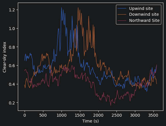
The relationship between space and time in the model occurs due to cloud advection. The cloud speed and direction, along with the spatial positions of the sites, determine the temporal correlation between sites. With a cloud_spd of 1 m/s and a cloud direction of 0 degrees, the cloud is moving eastward at 1 m/s. The two sites are arranged in the cloud direction 450 m spacing. This means that there will be a perfect correlation between the sites with a delay of 450 seconds, as visible by the delay between the two time series in the plot.

The third site is separated perpendicular to the cloud direction, so it will have a lower correlation with the other two sites, though it maintains some simultaneity with the upwind site.

cloud_spd = 1
cloud_dir = 0 * np.pi / 180

# Hourly clearsky
mean_csi = 0.52

e_pos = np.array([ 0, 450, 0])
n_pos = np.array([ 0,   0, 450])

times = pd.date_range(start='2024-01-01 00:00:00', end='2024-01-01 00:59:59', freq='15s')

c = downscale(times, e_pos, n_pos, cloud_spd, cloud_dir, mean_csi, DEFAULT_PARAMS, seed=42, scale=True, noneg=True)

plt.plot((times-times[0]).total_seconds(), c, linewidth=1, alpha=0.8)
plt.xlabel("Time (s)")
plt.ylabel("Clear-sky index")
plt.legend(['Upwind site', 'Downwind site', 'Northward Site']);

Cloud Field Visualizations

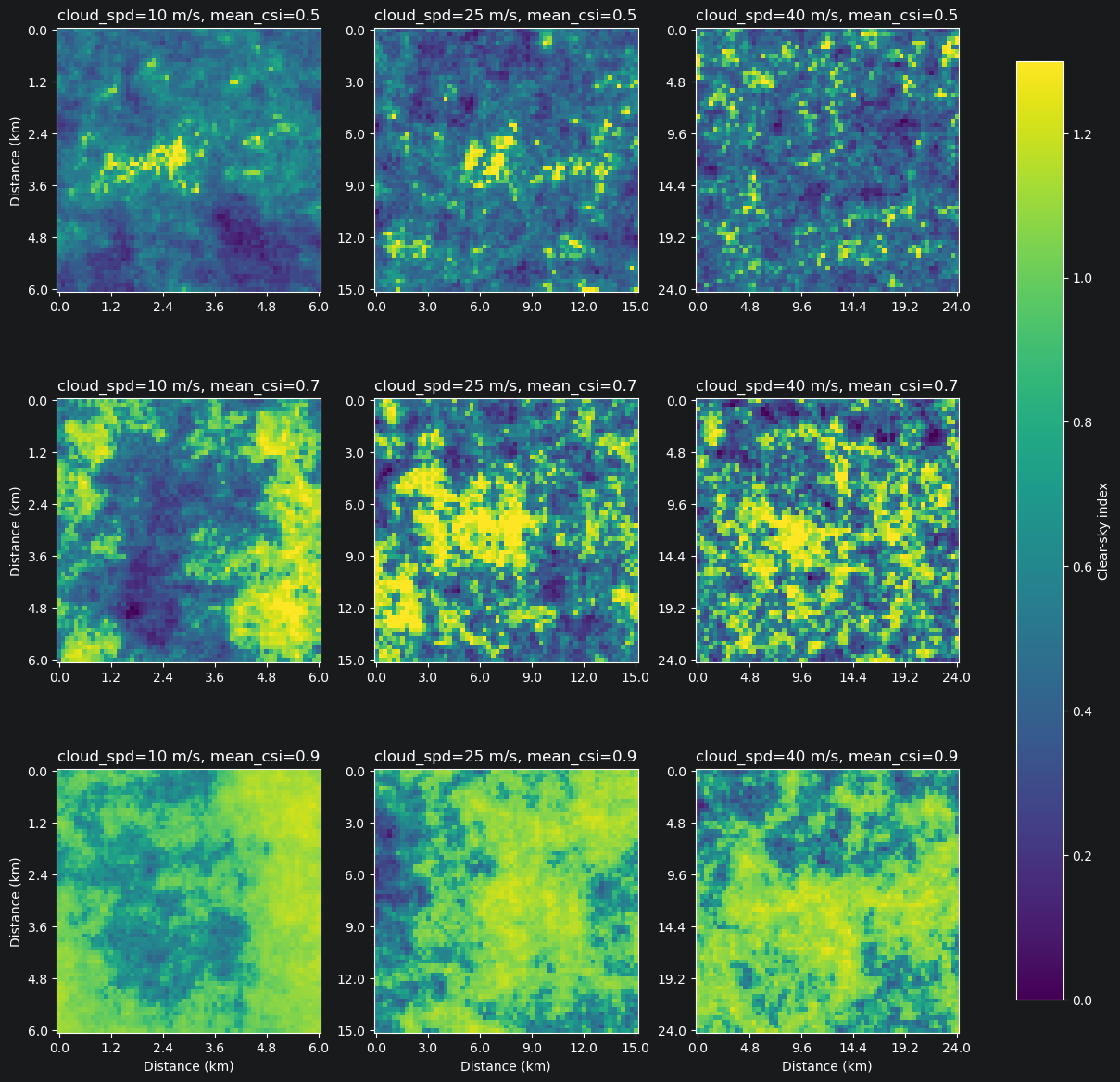
We don’t actually need to generate cloud fields using this method. Instead, we can just generate the individual time series for each sensor located within the field. However, we could generate a sample cloud field by evaluating the model on a rake of points in one direction (e.g. north-south) with a perpendicular (e.g. east) cloud direction. By making the spacing of the rake equal to the cloud speed times the time step, we actually produce a field of equally spaced sensors in both axes.

Sample cloud field plots for a range of cloud speeds and mean clear-sky index values are shown below. Because we maintain the number of pixels in each direction, varying the cloud speed essentially affects the zoom level of the field. Higher cloud speeds mean greater travel for the same dt, which means that the same number of pixels covers a larger area. This can be seen both in the axes and in the images, which depict smaller spatial scale of cloud features for higher cloud speeds. The mean clear-sky index affects the overall brightness of the field, with higher values producing brighter fields.

n = 60  # Num pixels in each axis
dt = 10  # Time step in seconds
cloud_dir = 0  # Cloud direction (east)
cloud_spd_vals = [10, 25, 40]  # cloud speed in m/x
mean_csi_vals = [0.5, 0.7, 0.9]  # mean clear-sky index

# Compute the time vector to maintain a size of n, with a spacing of dt
end_time = (pd.to_timedelta(f'{dt}s') * n).total_seconds()
times = pd.date_range(start='2024-01-01 00:00:00', end=f'2024-01-01 {int(end_time//3600):02d}:{int((end_time-(end_time//3600)*3600)//60):02d}:{int(end_time-(end_time//60)*60):02d}', freq=f'{dt}s')

fig, axes = plt.subplots(3, 3, figsize=(12, 12), constrained_layout=True)
tick_idx = np.arange(len(times))[::max(1, n // 5)]

for row, mean_csi in enumerate(mean_csi_vals):
    for col, cloud_spd in enumerate(cloud_spd_vals):

        # Compute the x & y position values such that we form a north-south rake with perpendicular motion
        # The vertical spacing should be equal to the spatiotemporal spacing implied by advection.
        e_pos = np.zeros(len(times))
        n_pos = np.arange(len(times)) * cloud_spd * dt

        # Downscale
        c = downscale(times, e_pos, n_pos, cloud_spd, cloud_dir, mean_csi, DEFAULT_PARAMS, seed=42, scale=True, noneg=True)

        ax = axes[row, col]
        im = ax.imshow(c, vmin=0, vmax=1.3)
        ax.set_aspect('equal')
        ax.set_xticks(tick_idx)
        ax.set_yticks(tick_idx)
        ax.set_xticklabels(n_pos[tick_idx] / 1000)
        ax.set_yticklabels(n_pos[tick_idx] / 1000)
        ax.set_title(f'cloud_spd={cloud_spd} m/s, mean_csi={mean_csi}')

for ax in axes[-1, :]:
    ax.set_xlabel('Distance (km)')

for ax in axes[:, 0]:
    ax.set_ylabel('Distance (km)')

fig.colorbar(im, ax=axes, label='Clear-sky index', shrink=0.85);

Multihour Downscaling

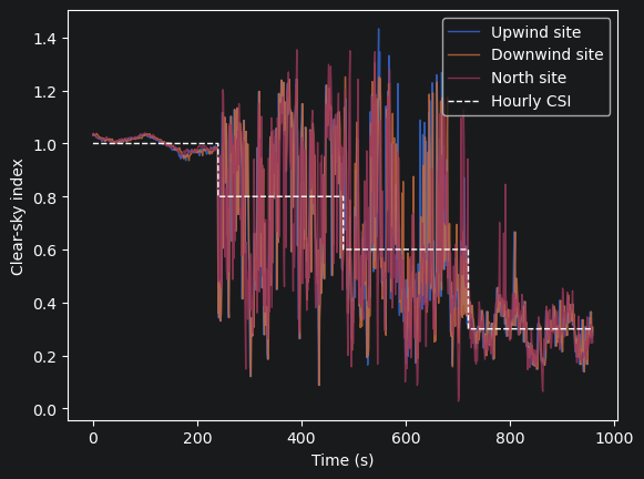
We can generate the time series for multiple hours with variable statistical properties using the copula.downscale_multihour function. The inputs are the same as for copula.downscale, except that the mean_csi, cloud_spd and cloud_dir parameters may now be a 1D array of values for each hour (or other sensible time period). In this case, times represents the time intervals for a single period of the measurement.

The function will generate a unique time series for each site for each time period with the corresponding statistical properties, while concatenating them into a single overall time series. Note that no matching occurs between periods, meaning that there may be discontinuities that occur at the boundaries.

cloud_spd = np.array([5, 30, 25, 15])
cloud_dir = np.zeros_like(cloud_spd)

# Hourly clearsky
mean_csi = np.array([1.0, 0.8, 0.6, 0.3])

e_pos = np.array([ 0, 450, 0])
n_pos = np.array([ 0,   0, 450])

times = pd.date_range(start='2024-01-01 00:00:00', end='2024-01-01 00:59:59', freq='15s')

c = downscale_multihour(times, e_pos, n_pos, cloud_spd, cloud_dir, mean_csi, DEFAULT_PARAMS, seed=42, scale=True, noneg=True)

csi_block = np.repeat(mean_csi, times.shape[0])

plt.plot(c, alpha=0.8, linewidth=1)
plt.step(np.arange(csi_block.size), csi_block, where='post', color='w', linewidth=1, linestyle='--', label='Hourly CSI')
plt.xlabel("Time (s)")
plt.ylabel("Clear-sky index")
plt.legend(['Upwind site', 'Downwind site', 'North site', 'Hourly CSI']);