Generating Synthetic Time Series Using Randomized Cloud Fields

This file demonstrates code available in solarspatialtools.synthirrad.cloudfield, which implements methods described by Lave et al. [1] for generation of synthetic cloud fields that can be used to simulate high frequency solar irradiance data. Some aspects of the implementation diverge slightly from the initial paper to follow a subsequent code implementation of the method shared by the original authors.

[1] Matthew Lave, Matthew J. Reno, Robert J. Broderick, “Creation and Value of Synthetic High-Frequency Solar Inputs for Distribution System QSTS Simulations,” 2017 IEEE 44th Photovoltaic Specialist Conference (PVSC), Washington, DC, USA, 2017, pp. 3031-3033, doi: https://dx.doi.org/10.1109/PVSC.2017.8366378.

Setup

Perform needed imports

import pvlib
import pandas as pd
import numpy as np
import matplotlib.pyplot as plt

from solarspatialtools import irradiance
from solarspatialtools import cmv
from solarspatialtools import spatial

from solarspatialtools.synthirrad.cloudfield import get_timeseries_stats, cloudfield_timeseries

Load Sample Timeseries Data

The model attempts to create representative variability to match that observed from a reference time series. In this case, we’ll process one of the 1-second resolution timeseries from the HOPE-Melpitz campign. We will load the data and convert it to clearsky index.

datafn = "data/hope_melpitz_1s.h5"
twin = pd.date_range('2013-09-08 9:15:00', '2013-09-08 10:15:00', freq='1s', tz='UTC')
data = pd.read_hdf(datafn, mode="r", key="data")

# Load the sensor positions
pos = pd.read_hdf(datafn, mode="r", key="latlon")
pos_utm = pd.read_hdf(datafn, mode="r", key="utm")

# Compute clearsky ghi and clearsky index
loc = pvlib.location.Location(np.mean(pos['lat']), np.mean(pos['lon']))
cs_ghi = loc.get_clearsky(data.index, model='simplified_solis')['ghi']
cs_ghi = 1000/max(cs_ghi) * cs_ghi # Normalize to 1000 W/m^2
kt = irradiance.clearsky_index(data, cs_ghi, 2)

For some of the later analysis, we will need to know something about the Cloud Motion Vector for this time period, so we can compute that using the solarspatialtools.cmv module.

cld_spd, cld_dir, _ = cmv.compute_cmv(kt, pos_utm, reference_id=None, method='jamaly')
cld_vec_rect = spatial.pol2rect(cld_spd, cld_dir)

print(f"Cld Speed  {cld_spd:8.2f}, Cld Dir {np.rad2deg(cld_dir):8.2f}°")

Cld Speed     19.67, Cld Dir    90.70°

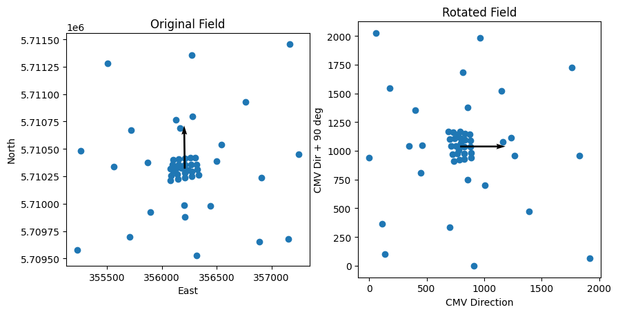
Visualize the sensor layout in the CMV direction

We want to describe how the sensors are distributed in the cloud motion vector direction. So we’ll rotate the positions of the entire field to align with the CMV in the +X direction. This will allow us to describe positions of sensors within the field with respect to the motion of clouds, which seldom aligns with the cardinal directions.

# Rotation by -cld_dir to make CMV align with X Axis
rot = spatial.rotate_vector((pos_utm['E'], pos_utm['N']), theta=-cld_dir)
pos_utm_rot = pd.DataFrame({'X': rot[0] - np.min(rot[0]), 'Y': rot[1] - np.min(rot[1])}, index=pos_utm.index)

fig, axs = plt.subplots(1, 2, figsize=(10, 5))
axs[0].scatter(pos_utm['E'], pos_utm['N'])
axs[0].set_title('Original Field')
axs[0].quiver(pos_utm['E'][40], pos_utm['N'][40], 200 * cld_vec_rect[0], 200 * cld_vec_rect[1], scale=10, scale_units='xy')
axs[0].set_xlabel('East')
axs[0].set_ylabel('North')
axs[1].scatter(pos_utm_rot['X'], pos_utm_rot['Y'])
axs[1].quiver(pos_utm_rot['X'][40], pos_utm_rot['Y'][40], 200*cld_spd, 0, scale=10, scale_units='xy')
axs[1].set_title('Rotated Field')
axs[1].set_xlabel('CMV Direction')
axs[1].set_ylabel('CMV Dir + 90 deg')
axs[0].set_aspect('equal')
axs[1].set_aspect('equal')

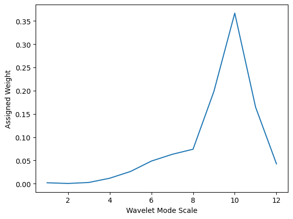
Compute Timeseries Statistics

The scaling of the cloud field is based on variability as expressed through statistical properties of the time series. So we’ll extract those in advance. We do so for a single sensor (number 40) that is centrally located in the field, though more detailed analysis could consider representing properties for the entire field. - ktmean - The mean clearsky index - kt1pct - The 1st percentile of clearsky index, used similar to a minimum - ktmax - The maximum clearsky index (shows cloud enhancement) - frac_clear - Fraction of clear sky conditions in time series (characterized as kt > 0.95) - vs - The variability score of the clearsky index - weights - The weights are calculated from the magnitude-squared of the various wavelet modes contained in the time series. - scales - The scales of the various wavelet modes contained in the time series.

ktmean, kt1pct, ktmax, frac_clear, vs, weights, scales = get_timeseries_stats(kt[40], plot=False)
print(f"ktmean: {ktmean:8.2f}")
print(f"kt1pct: {kt1pct:8.2f}")
print(f"ktmax: {ktmax:8.2f}")
print(f"frac_clear: {frac_clear:8.2f}")
print(f"vs: {vs:8.2f}")

# Plot the wavelet scales
plt.plot(scales, weights)
plt.xlabel('Wavelet Mode Scale')
plt.ylabel('Assigned Weight')
plt.show()

ktmean:     0.64
kt1pct:     0.38
ktmax:     1.09
frac_clear:     0.12
vs:    25.31

Relate the Time and Space Scales

Since we rotated the sensor positions, we can now calculate the overall spatial size of the distribution along and perpendicular to the cloud motion vector. We’ll also look at the dureation of the time series (in this case 1 hour) and its temporal resolution (1 second).

Using the cloud speed we can relate these spatial dimensions to time dimensions. When we generate the cloud field, we will assume that each pixel in the field represents a 1-second step in time. So moving 1 pixel within the field along the X axis represents either a 1 second shift upwind or downwind in space, or a 1 second shift of the time axis at a fixed spatial position as clouds transit the field. Moving 1 pixel along the Y axis will always represent a 1 second spatial shift perpendicular to the cloud motion vector, since no motion occurs in that direction.

x_extent = np.abs(np.max(pos_utm_rot['X']) - np.min(pos_utm_rot['X']))
y_extent = np.abs(np.max(pos_utm_rot['Y']) - np.min(pos_utm_rot['Y']))
t_extent = (np.max(twin) - np.min(twin)).total_seconds()
dt = (twin[1] - twin[0]).total_seconds()

spatial_time_x = x_extent / cld_spd
spatial_time_y = y_extent / cld_spd

xt_size = int(np.ceil(spatial_time_x + t_extent))
yt_size = int(np.ceil(spatial_time_y))

print(f"X Extent: {x_extent:8.2f} m, Y Extent: {y_extent:8.2f} m")
print(f"Time Extent: {t_extent:8.2f} s, Time Resolution: {dt:8.2f} s")
print(f"Field Size: {xt_size}x{yt_size}")

X Extent:  1919.58 m, Y Extent:  2023.44 m
Time Extent:  3600.00 s, Time Resolution:     1.00 s
Field Size: 3698x103

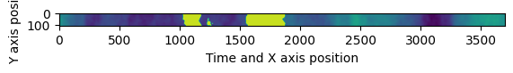
Generating the Randomized Cloud Field

The function cloudfield_timeseries generates a cloud field from which time series can be sampled. The field is generated by creating a random field of cloudiness, then scaling it to match the clear sky condition properties of the reference time series. The output field’s first axis (rows) represents the spatial dimension perpendicular to the cloud motion vector. The second axis (columns) represent the spatial dimension along the cloud motion vector, which coincides with time axis.

Each pixel represents a time step of 1 second, either in literal time, or associated with a spatial shift of the equivalent of 1 second of cloud motion. In this case, where the cloud velocity is around 20 m/s, this implies that a shift along either axis corresponds to a 20 m spatial shift.

np.random.seed(42)  # Seed for repeatability

field_final = cloudfield_timeseries(weights, scales, (xt_size, yt_size), frac_clear, ktmean, ktmax, kt1pct)

plt.imshow(field_final.T, aspect='equal', cmap='viridis')
plt.xlabel('Time and X axis position')
plt.ylabel('Y axis position')
plt.show()

Extracting the time series at a point

We can extract the time series at points in the field. We need to first convert our spatial positions into a spatially based coordinate system. We can then choose that starting point as a location for a time series at that point. The time series will extend along the x-axis with each time series at a length of t_extent seconds.

One consequence of this approach that is important to note is that any two points that are located precisely up/down-wind from each other will have identical time series, albeit with a delay associated with the cloud motion. This is visible in the results below in which the two sensors are nearly aligned with the cloud motion, but have an upwind/downwind separation.

# Convert space to time to extract time series
xpos = pos_utm_rot['X'] - np.min(pos_utm_rot['X'])
ypos = pos_utm_rot['Y'] - np.min(pos_utm_rot['Y'])
xpos_temporal = xpos / cld_spd
ypos_temporal = ypos / cld_spd

# Extract simulated time series at all sensor positions
sim_kt = pd.DataFrame(index=twin, columns=pos_utm_rot.index)
for sensor in pos_utm_rot.index:
    # Negate X positions for upwind/downwind positions, so that downwind shows later
    x = int(max(xpos_temporal) - xpos_temporal[sensor])
    y = int(ypos_temporal[sensor])

    # Select a time series of length t_extent starting at the x,y position
    sim_kt[sensor] = field_final[x:x+int(t_extent)+1, y]

# Create two side by side figures
fig, axs = plt.subplots(1, 2, figsize=(12, 5))
axs[0].plot(sim_kt[[60, 70]])
axs[0].set_xlabel('Time (s)')
axs[0].set_ylabel('Clearsky Index')
axs[0].legend(['Upwind', 'Downwind'])
import matplotlib.dates as mdates
myFmt = mdates.DateFormatter('%H:%M')
axs[0].xaxis.set_major_formatter(myFmt)

axs[1].scatter(pos_utm_rot['X'], pos_utm_rot['Y'])
axs[1].scatter(pos_utm_rot['X'][[60,70]], pos_utm_rot['Y'][[60,70]], color='r')
for i, txt in enumerate([60, 70]):
    axs[1].annotate(txt, (pos_utm_rot['X'][txt], pos_utm_rot['Y'][txt]))
    axs[1].quiver(pos_utm_rot['X'][40], pos_utm_rot['Y'][40], 200*cld_spd, 0, scale=10, scale_units='xy')
axs[1].set_aspect('equal')
axs[1].set_xlabel('X Position')
axs[1].set_ylabel('Y Position')
plt.show()

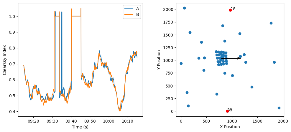
Two sensors that are separated in the perpendicular direction to the motion experience differences in the time series due to spatial position discrepancies, but would see large scale phenomena at the same time. In part, that’s because the weights for this particular cloud field are biased towards large scales.

# Create two side by side figures
fig, axs = plt.subplots(1, 2, figsize=(12, 5))
axs[0].plot(sim_kt[[18, 38]])
axs[0].set_xlabel('Time (s)')
axs[0].set_ylabel('Clearsky Index')
axs[0].legend(['A', 'B'])
import matplotlib.dates as mdates
myFmt = mdates.DateFormatter('%H:%M')
axs[0].xaxis.set_major_formatter(myFmt)

axs[1].scatter(pos_utm_rot['X'], pos_utm_rot['Y'])
axs[1].scatter(pos_utm_rot['X'][[18,38]], pos_utm_rot['Y'][[18,38]], color='r')
for i, txt in enumerate([18, 38]):
    axs[1].annotate(txt, (pos_utm_rot['X'][txt], pos_utm_rot['Y'][txt]))
    axs[1].quiver(pos_utm_rot['X'][40], pos_utm_rot['Y'][40], 200*cld_spd, 0, scale=10, scale_units='xy')
axs[1].set_aspect('equal')
axs[1].set_xlabel('X Position')
axs[1].set_ylabel('Y Position')
plt.show()

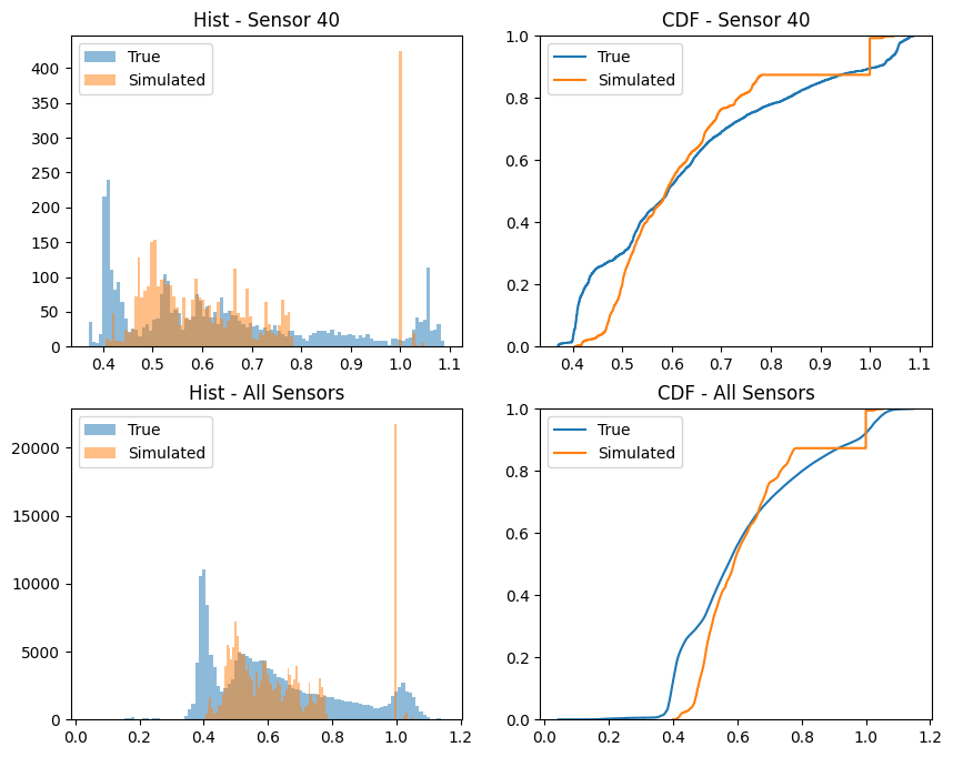
It might also be interesting to compare the statistical distribution of the true and simulated timeseries. We can do this by comparing the histograms and CDFs of the two time series.

# show histograms and CDFs
fig, axs = plt.subplots(2, 2, figsize=(10, 8))
axs[0,0].hist(kt[40], bins=100, alpha=0.5, label='True')
axs[0,0].hist(sim_kt[40], bins=100, alpha=0.5, label='Simulated')
axs[0,0].legend()
axs[0,0].set_title('Hist - Sensor 40')
axs[0,1].ecdf(kt[40], label='True')
axs[0,1].ecdf(sim_kt[40], label='Simulated')
axs[0,1].set_title('CDF - Sensor 40')
axs[0,1].legend()
axs[1,0].hist(kt.values.flatten(), bins=100, alpha=0.5, label='True')
axs[1,0].hist(sim_kt.values.flatten(), bins=100, alpha=0.5, label='Simulated')
axs[1,0].legend()
axs[1,0].set_title('Hist - All Sensors')
axs[1,1].ecdf(kt.values.flatten(), label='True')
axs[1,1].ecdf(sim_kt.values.flatten(), label='Simulated')
axs[1,1].set_title('CDF - All Sensors')
axs[1,1].legend()
plt.show()

Appendix - Internal methodology of the cloud field generation

It’s worth looking in more detail at the internal processes of the cloud generation methodology to better understand what’s happening.

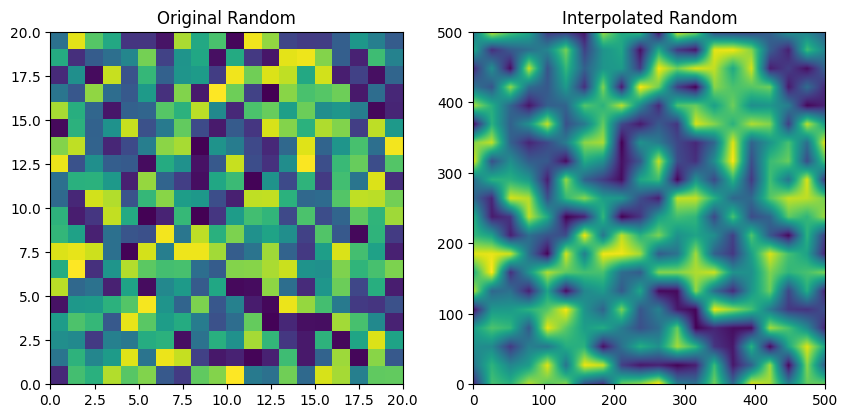
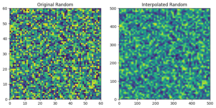
Cloud field relies on generating various scales of random noise and adding them together. The job of the function _random_at_scale is to generate a random field at a given scale and then interpolate it to a higher resolution. This function will be called at each level of the wavelet decomposition to generate the cloud field with different scaling factors.

from solarspatialtools.synthirrad.cloudfield import _stack_random_field, _calc_clear_mask, _find_edges, _scale_field_lave, _random_at_scale

np.random.seed(42)
layer, interp_layer = _random_at_scale((20, 20), (500, 500), plot=True)
layer, interp_layer = _random_at_scale((60, 60), (500, 500), plot=True)

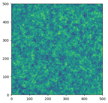
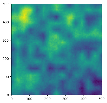
We’ll now show two examples of _stack_random_field that will combine multiple such layers, stacked field across the multiple scales/weights. The first example will show the cloud field generated with a bias toward small scales (high variability) while the second will show a cloud field generated with predominantly large scales (low variability).

internal_size = (500, 500)
fine_weights = np.array([1, 1, 1, 1, 1, 0.1, 0.1, 0.1, 0.1, 0.1])
coarse_weights = np.flipud(fine_weights)
scales = np.array([1, 2, 3, 4, 5, 6, 7, 8, 9, 10])

internal_cfield = _stack_random_field(fine_weights, scales, internal_size, plot=True)
internal_cfield = _stack_random_field(coarse_weights, scales, internal_size, plot=True)

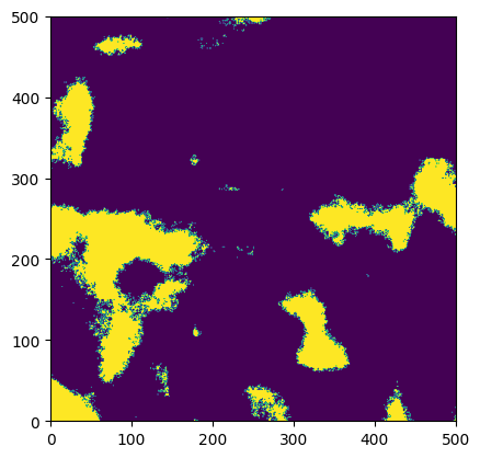
Directly using these fields isn’t realistic, because they doesn’t produce roughly normally distributed noise, rather than a cloudy/clear dichotomy like we would see in a real sky. So we will create an additional random field that will be used to create a mask. The reson we don’t just mask the field directly is that we want to ensure that the variability isn’t self-correlated to the shape of the clouds. First we will create a new random field, and then we will specify a fraction of clear sky conditions that we wish to have. Because the stacked field is not a uniform distribution, we will set a threshold level based on quantile within the field, as implemented by _calc_clear_mask.

frac_clear = 0.15
internal_clear_mask = _stack_random_field(coarse_weights, scales, internal_size)
internal_clear_mask = _calc_clear_mask(internal_clear_mask, frac_clear, plot=True)  # 0 is cloudy, 1 is clear

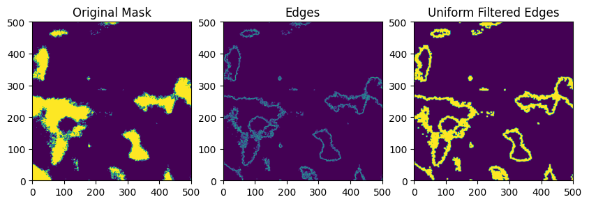
Additionally, we will find edges in the clear mask. This will be used to create an additional edge mask that will be used to apply cloud enhancement at the edges of the cloudy regions. The edgesmoothing parameter will control an amount of smoothing that is applied to the edge mask, which helps to decide how wide the cloud edges should be. Edge smoothing essentially performs a dilation operation on the edge mask.

internal_edgesmoothing = 3
edges, smoothed = _find_edges(internal_clear_mask, internal_edgesmoothing, plot=True)

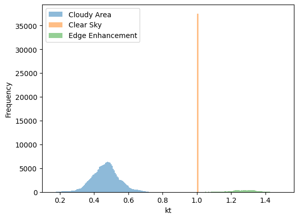
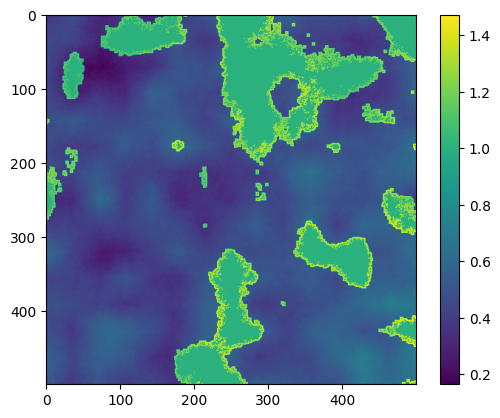
We do some scaling to make the final field have the desired statistical properties. This happens in several steps. 1) Scale the field to be distributed from from kt1pct to the 99th percentile of the field, since we never see real values of kt approach zero. Clip this distribution to [0, 1] just in case there are entries outside the bounds. This transforms our field to represent the clear sky index ranging from the 1pct to 1.0, representing values of the clear sky index. 2) Calculate a copy of this field and scale it to range from 1 to ktmax. This will be used to represent the cloud enhancement. 3) Select only the regions of the final mask that will be cloudy (i.e. exclude the values of the field that are clear sky (and thus have a value of 1) and the edge enhanced regions). Calculate a scaling factor such that the mean of the cloudy region will lead to a global field mean of ktmean. 4) Apply the cloud enhancement field values to the regions assigned as edges. 5) Assign a value of 1 to the clear sky regions (note that the order of 4 & 5 ensures that the cloud enhancement stops sharply at the cloud edges).

The distribution will basically have three sub regions: clear sky (always 1), cloud enhancement edges (range from 1 to ktmax) and cloudy regions (range is scaled to produce desired ktmean). The overall mean of the field will be ktmean, and the maximum value will be close to ktmax. Note that kt1pct may not be respected in the final distribution, but instead follows the original author’s implementation of the method.

ktmean = 0.6
kt1pct = 0.2
ktmax = 1.5

internal_field_final = _scale_field_lave(internal_cfield, internal_clear_mask, smoothed, ktmean, ktmax, kt1pct)
print(f"ktmean: {np.mean(internal_field_final):8.2f}")
print(f"kt1pct: {np.min(internal_field_final):8.2f}")
print(f"ktmax: {np.max(internal_field_final):8.2f}")

plt.hist(internal_field_final.flatten()[internal_field_final.flatten()<1], bins=100, alpha=0.5)
plt.hist(internal_field_final.flatten()[internal_field_final.flatten()==1], bins=100, alpha=0.5)
plt.hist(internal_field_final.flatten()[internal_field_final.flatten()>1], bins=100, alpha=0.5)
plt.legend(["Cloudy Area", "Clear Sky", "Edge Enhancement"])
plt.ylabel('Frequency')
plt.xlabel('kt')

plt.figure()
plt.imshow(internal_field_final.T, aspect='equal', cmap='viridis')
plt.colorbar()
plt.show()

ktmean:     0.60
kt1pct:     0.16
ktmax:     1.47

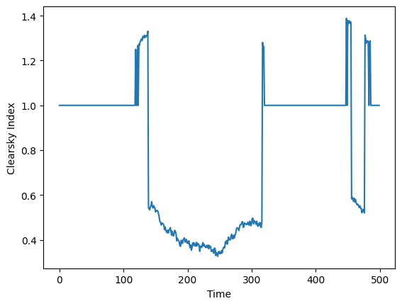
We can now see an example time series.

plt.plot(internal_field_final[250, :])
plt.xlabel('Time')
plt.ylabel('Clearsky Index')
plt.show()

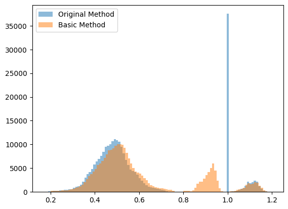
There’s also an alternate scaling method available that contains a few additional options, including the ability to have the clearsky values reflect a distribution rather than uniform 1 values. This is implemented in the function _scale_field_basic.

from solarspatialtools.synthirrad.cloudfield import _scale_field_basic

# We compare using flipdistr=True on the basic method, because the lave method uses the flipping.
internal_field_final = _scale_field_lave(internal_cfield, internal_clear_mask, smoothed, 0.6, 1.2, 0.2)
internal_field_final2 = _scale_field_basic(internal_cfield, internal_clear_mask, smoothed, 0.6, 1.2, 0.2, flipdistr=True, cs_smoothing=0.8)

# Display a comparative histogram
plt.hist(internal_field_final.flatten(), bins=100, alpha=0.5, label='Original Method')
plt.hist(internal_field_final2.flatten(), bins=100, alpha=0.5, label='Basic Method')
plt.legend()
plt.show()

# Display the fields and the time series
fig, axs = plt.subplots(2, 2, figsize=(10, 8))
axs[0,0].imshow(internal_field_final, extent=(0, internal_field_final.shape[1], 0, internal_field_final.shape[0]))
axs[0,0].set_title('Original Scaling')
axs[0,1].imshow(internal_field_final2, extent=(0, internal_field_final2.shape[1], 0, internal_field_final2.shape[0]))
axs[0,1].set_title('Modified Scaling')
# plot a time series from each
axs[1,0].plot(internal_field_final[0, :], label='Original Method')
axs[1,1].plot(internal_field_final2[0, :], label='Basic Method')
plt.show()

# compare the statistics of max and min from the two methods
print(f"Original Method: Max {internal_field_final.max():.2f}, Min {np.quantile(internal_field_final.flatten(), 0.01):.2f}, Mean {internal_field_final.mean():.2f}")
print(f"Basic Method: Max {internal_field_final2.max():.2f}, Min {np.quantile(internal_field_final2.flatten(), 0.01):.2f}, Mean {internal_field_final2.mean():.2f}")

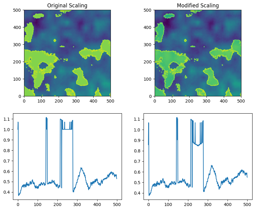
Original Method: Max 1.19, Min 0.28, Mean 0.60
Basic Method: Max 1.20, Min 0.28, Mean 0.60