Field Analysis Demo

Field analysis is a calculation method that is intended for validating the expected locations of various discrete plant components (e.g. combiners). It identifies cloud motion within the individual component time series and infers their positions based upon relative timing of the cloud signal to each individual component. A full description of the technique is available in a paper: J. Ranalli and W. Hobbs, PV Plant Equipment Labels and Layouts can be Validated by Analyzing Cloud Motion in Existing Plant Measurements, Submitted to IEEE Journal of Photovoltaics.

This demo utilizes sample data on a single plant to demonstrate the application of the method.

[1]:

import pandas as pd
import numpy as np
import matplotlib.pyplot as plt

from solarspatialtools import spatial, field

Read the Data

The sample data file is a compressed H5 file that contains all the info used to perform the analysis.

The Plant Layout

The layout of the plant is placed in the variable pos_utm. Its definition is contained in the field latlon, which produces a DataFrame of the combiner centroids in a UTM-like coordinate system. It contains combiner IDs as the index, and columns E and N that indicate the mean position of the combiner footprint (i.e. the centroid). The combiners are named following the pattern CMB-<INVERTER#>-<COMBINER#>.

[2]:

datafile = "data/sample_plant_2.h5"
pos_utm = pd.read_hdf(datafile, mode="r", key="utm")
pos_utm

[2]:

	E	N
CMB-001-1	23.584970	1086.290244
CMB-001-2	49.679324	1086.290365
CMB-001-3	84.519736	1086.290633
CMB-001-4	125.324187	1086.291124
CMB-001-5	160.281453	1086.291697
...	...	...
CMB-048-4	695.084107	31.788344
CMB-048-5	729.924241	31.791192
CMB-048-6	764.894729	31.794191
CMB-048-7	799.739358	31.797319
CMB-048-8	831.869055	31.800323

382 rows × 2 columns

The Time Series Data

The method relies on two discrete time periods with a fixed CMV. Two examples are stored in the data file with keys data_a and data_b. These each represent one hour of data for each combiner in the plant with a 10s sampling resolution. The DataFrames are indexed by a time that is artificially offset to begin at a time of 00:00:00 on an arbitrary day. The columns of the DataFrames have keys that match the index of pos_utm.

[3]:

ts_data_a = pd.read_hdf(datafile, mode="r", key="data_a")
ts_data_b = pd.read_hdf(datafile, mode="r", key="data_b")
ts_data_a

[3]:

	CMB-001-1	CMB-001-2	CMB-001-3	CMB-001-4	CMB-001-5	CMB-001-6	CMB-001-7	CMB-002-1	CMB-002-2	CMB-002-3	...	CMB-047-7	CMB-047-8	CMB-048-1	CMB-048-2	CMB-048-3	CMB-048-4	CMB-048-5	CMB-048-6	CMB-048-7	CMB-048-8
2023-01-01 00:00:00	93.799402	93.985920	93.622077	94.318063	93.390276	93.459779	93.753268	95.253145	95.510679	95.718582	...	92.871630	92.798612	91.074627	91.385004	91.554207	91.528461	91.404796	91.747153	91.461591	91.606280
2023-01-01 00:00:10	94.508405	94.819152	95.028923	95.105311	93.855248	94.410892	94.540710	95.633790	95.760610	95.699990	...	92.753680	92.873880	91.292149	91.850400	91.644421	91.739311	91.842573	91.653509	91.475838	91.425386
2023-01-01 00:00:20	94.767218	95.245977	95.438032	95.826806	94.000549	94.737096	94.925867	95.603580	95.745574	95.265605	...	92.933072	92.732030	91.251834	91.799432	91.926831	91.726960	91.657963	91.725119	91.453577	91.490994
2023-01-01 00:00:30	94.880949	95.406670	95.139340	95.771861	94.032838	94.730620	95.055108	95.470650	95.914626	96.075220	...	92.942349	92.877739	91.443098	92.072665	91.937813	91.629913	91.534880	91.854972	91.431316	91.431947
2023-01-01 00:00:40	94.837813	95.538455	95.515880	95.826806	94.407401	94.698243	95.155677	95.337730	95.736634	95.525902	...	92.886374	92.751329	91.496539	92.014166	91.867211	91.532872	91.664974	91.688921	91.409054	91.577226
...	...	...	...	...	...	...	...	...	...	...	...	...	...	...	...	...	...	...	...	...	...
2023-01-01 00:59:20	14.373001	13.225903	14.791491	13.385478	13.085343	13.466051	14.118774	13.721180	13.306969	8.306490	...	14.580523	15.408295	14.735548	15.268503	15.645326	17.442542	17.913292	17.870185	16.114405	16.653684
2023-01-01 00:59:30	14.583977	13.338135	14.856895	13.349449	13.317424	13.456741	14.205222	13.811406	13.327289	8.690166	...	14.611648	15.615766	14.689607	14.798921	14.540775	16.176576	18.011441	18.704340	17.892674	19.351115
2023-01-01 00:59:40	14.610643	13.486927	14.896615	13.516509	13.312177	13.673675	14.273695	13.934259	13.347608	8.382548	...	14.247965	15.191175	14.563032	14.489767	14.585489	15.712535	15.359870	15.863494	18.463466	23.291351
2023-01-01 00:59:50	14.594957	13.737747	15.056860	13.734342	13.508587	13.867665	14.499656	13.958829	13.495051	8.701196	...	14.179527	14.860188	14.610850	14.564967	14.809852	15.814871	15.672231	16.217617	15.594370	17.694980
2023-01-01 01:00:00	14.933424	13.887485	15.247237	13.952175	13.770243	14.039324	14.641018	14.113163	13.674277	9.230496	...	14.203536	14.929559	14.533342	14.613296	14.461280	15.638823	15.624369	16.330934	15.905045	17.639993

361 rows × 382 columns

It’s necessary to provide the CMV for each time period. These precomputed values for the time periods in the data file are provided here. It’s also possible to compute them directly using methods in solarspatialtools.cmv. Note that it’s necessary for the CMVs to be roughly perpendicular, because the matrix calculation associated with triangulating the predicted position becomes singular for CMVs that are too close to parallel (or anti-parallel).

One other potential issue with CMVs is that the spatialsolartools.cmv module is also based on accurate knowledge of the combiner positions. In our experience, even plants with small numbers of scrambled combiners can still produce useful CMVs, because the position errors are averaged out when including all the combiners in the entire plant. A completely scrambled plant with no confidence in any of the combiner positions would likely require special handling, or CMVs from an independent source. But users should be aware of this as a potential limitation of the technique for very low confidence plant maps.

[4]:

cmv_a = spatial.pol2rect(9.52, 0.62)
cmv_b = spatial.pol2rect(8.47, 2.17)

Perform the Field Analysis

A high level execution of the field routine for a single CMV pair is performed by compute_predicted_position. This routine works on a single combiner at a time and on a single CMV pair at a time. Running it in a loop allows multiple combiners to be tested (only 10 points are shown here, due to computational time considerations). It returns a variable (pos) that holds the predicted position of the target combiner on the basis of other neighboring combiners that that serve as a spatial reference.

Results are stored in a new DataFrame (df).

[5]:

df = pd.DataFrame(index=pos_utm.index, columns=['E', 'N', 'com-E', 'com-N'])

for ref in pos_utm.index[46:62]:

    pos, _ = field.compute_predicted_position(
        [ts_data_a, ts_data_b],  # The dataframes with the two one hour periods
        pos_utm,  # the dataframe specifying the combiner positions
        ref,  # the combiner id to calculate the position for
        [cmv_a, cmv_b],  # The two individual CMVs for the DFs
        mode='preavg',  # Mode for downselecting the neighboring points
        ndownsel=8)  # Num points to use for downselecting

    # Add this combiner's calculated position to the output DataFrame
    df.loc[ref] = [pos_utm.loc[ref]['E'], pos_utm.loc[ref]['N'], pos[0], pos[1]]

Results

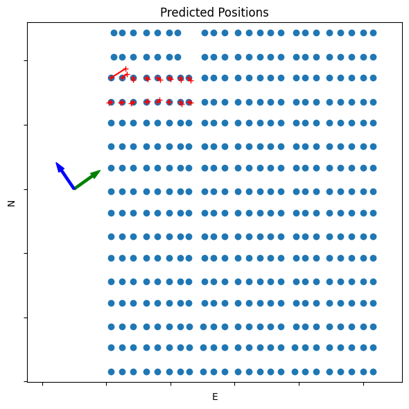
The following code generates a plot showing the location of the combiners in the entire plant. The red lines indicate the difference between the expected and calculated positions of the combiners tested. The CMVs for the two time periods are indicated by the green and blue arrows to the side of the plot.

The results shown here indicate combiners whose predicted position generally agrees with the expected position from the plant design. It can be helpful to repeat this calculation for different CMV pairs and to average the positions to determine the degree to which the predictions are repeatable and independent of the CMV.

[6]:

plt.figure(figsize=(6, 6))
plt.scatter(pos_utm['E'], pos_utm['N'])

for row in df.iterrows():
    r = row[1]
    plt.plot([r['E'], r['com-E']], [r['N'], r['com-N']], 'r-+')

# Plot some arrows to show the CMV
for cmv, color in zip([cmv_a, cmv_b],['green','blue']):
    velvec = np.array(spatial.unit(cmv)) * 100
    plt.arrow(-100, 600, velvec[0], velvec[1],
              length_includes_head=True, width=7, head_width=20, color=color)

plt.axis('equal')
plt.xlabel('E')
plt.ylabel('N')
plt.title(f'Predicted Positions')
axes = plt.gca()
axes.xaxis.set_ticklabels([])
axes.yaxis.set_ticklabels([])
plt.tight_layout()

plt.show()